Infram8 Labs · · 22 min read
Updated
By Infram8
A City Does Not Behave Like a Spreadsheet
How CNN-LSTM and CNN-GRU Connect Urban Sensors, Spatial-Temporal Deep Learning, and Intelligent Infrastructure
Abstract
Abstract
Urban systems are inherently spatial-temporal: traffic congestion propagates across road networks, pollutant concentrations shift with emissions and wind, and thermal gradients evolve through daily and seasonal cycles. Static dashboards, isolated sensor feeds, and tabular historical averages are structurally mismatched to these phenomena. This article examines how Convolutional Neural Network-Long Short-Term Memory (CNN-LSTM) and CNN-Gated Recurrent Unit (CNN-GRU) hybrid architectures address this mismatch by jointly modeling spatial patterns and temporal evolution in urban sensor data [1]-[4]. Five major smart-city application domains are examined: air quality prediction, urban heat island monitoring, traffic forecasting, energy demand forecasting, and predictive maintenance of urban infrastructure. The central argument is that the model is one layer in a broader system: the full chain from sensors to signal quality, telemetry, data pipelines, infrastructure, model outputs, uncertainty quantification, and operational decision-making determines whether spatial-temporal learning creates operational value. Limitations examined include sensor drift, spatial coverage bias, data missingness, model non-stationarity, interpretability constraints, and the risks of predictions made without uncertainty bounds. The article is intended for engineers, infrastructure architects, data scientists, and urban intelligence professionals seeking a scientifically grounded, architecturally mature perspective on spatial-temporal AI for cities.
Methodological Note
Methodological Note
This article is a literature-informed synthesis of architectural principles, published findings, and operational considerations for spatial-temporal deep learning in smart-city systems. It does not report original experimental results and does not claim that CNN-LSTM or CNN-GRU architectures outperform all alternatives on any specific benchmark or task. Reported application examples describe areas where these architectures have been studied in the literature; they do not imply guaranteed performance in any particular deployment. Architecture selection must be empirically validated for each specific dataset, domain, spatial resolution, temporal horizon, sensor configuration, and deployment context. Readers seeking benchmarking results are directed to the primary literature cited throughout the article.
Section 01
Introduction: A City Is Not a Spreadsheet
A city does not behave like a spreadsheet.
Spreadsheets can encode dependencies through formulas. The limitation is treating urban observations as independent rows, which can obscure the spatial dependencies and temporal dynamics that give those measurements context. Traffic congestion at one intersection ripples outward across the road network for hours. An industrial emission source shapes air quality readings kilometers away, depending on wind direction, atmospheric stability, and urban morphology. A thunderstorm that reaches one district at dawn reshapes energy demand, surface temperatures, and transport behavior across the entire metropolitan area before noon.
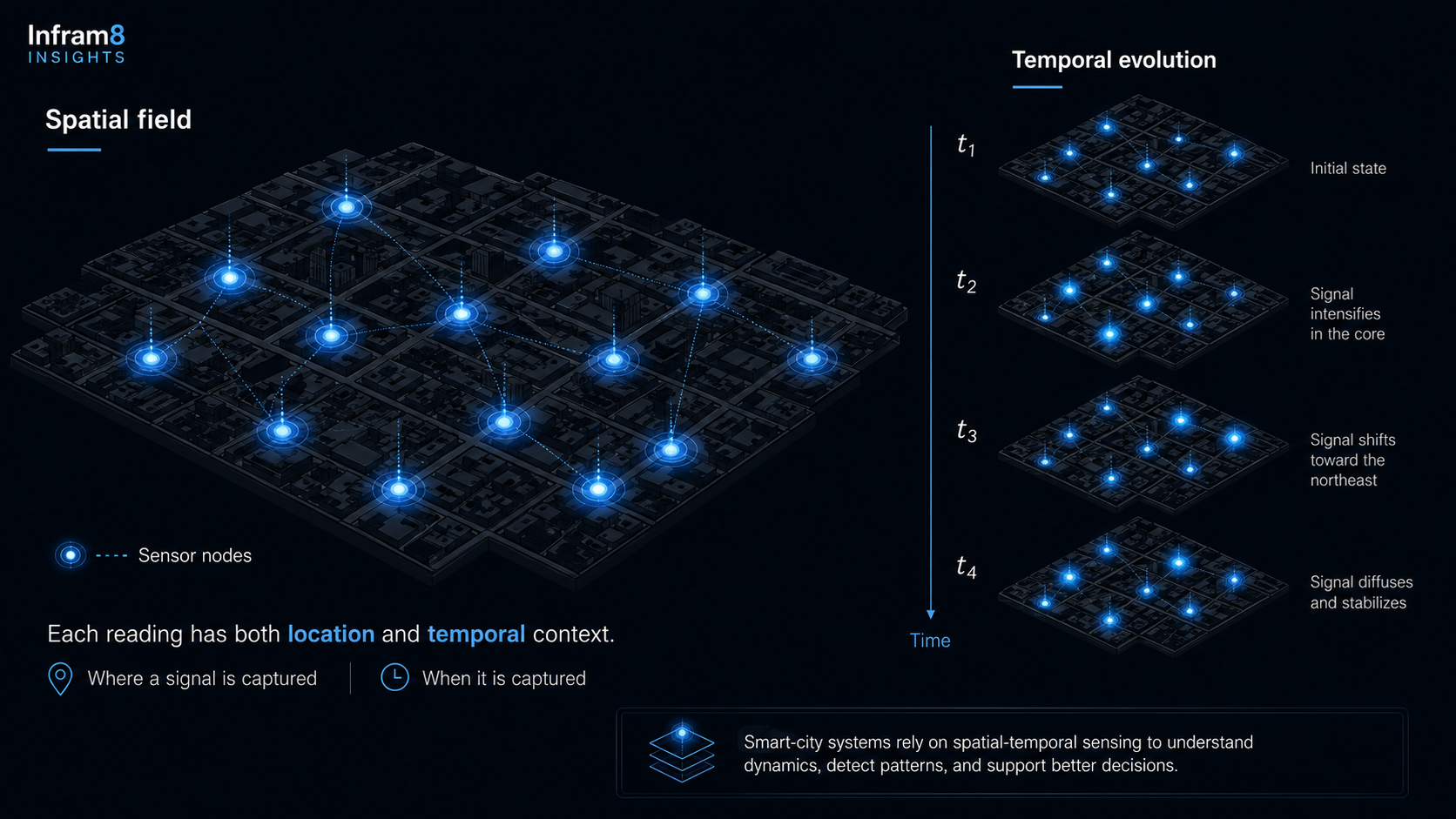
Urban systems generate spatial-temporal signals, not isolated data points. Every sensor embedded in a street, rooftop, vehicle, or building captures a fragment of a continuously evolving physical and social process. That fragment has meaning only when interpreted alongside its spatial neighbors and its temporal predecessors and successors [10].
This structural reality exposes a fundamental weakness in much of what currently passes for smart-city intelligence: the treatment of urban data as if it were a spreadsheet. Static dashboards. Isolated sensor feeds. Historical averages. Threshold alerts that fire when a single variable crosses a fixed boundary. Used without spatial and temporal context, these approaches can miss important dependencies in the phenomena they are meant to model.
Hybrid deep learning architectures, specifically CNN-LSTM and CNN-GRU models, offer a more structurally matched approach. These architectures combine the spatial feature-learning capacity of Convolutional Neural Networks [1] with the sequential memory of Long Short-Term Memory networks [2] or Gated Recurrent Units [3], enabling models that learn patterns evolving across both space and time. The seminal ConvLSTM architecture by Shi et al. (2015) established the viability of integrating convolutional and recurrent operations for spatially correlated sequence prediction [4], laying conceptual groundwork for a range of urban applications.
However, the most important argument in this article is not about model design. It is about system design. CNN-LSTM and CNN-GRU are one layer in a much longer chain:
The infrastructure chain
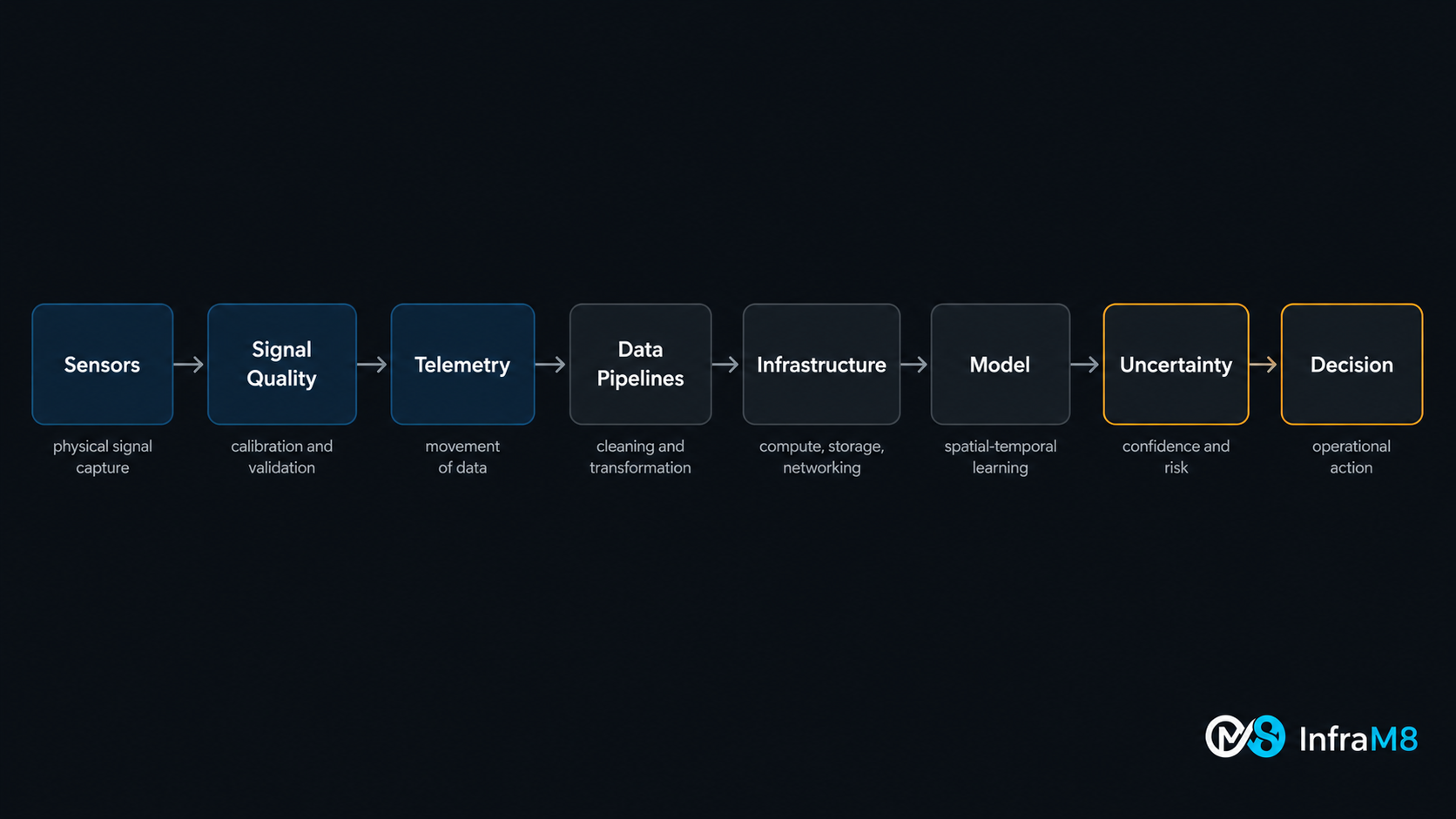
sensors -> signal quality -> telemetry -> data pipelines -> infrastructure -> model -> uncertainty -> decision
Every link in that chain conditions the usefulness of the model at its center. A spatially-temporally sophisticated architecture deployed on poorly calibrated sensors, fragile telemetry, or pipelines lacking data governance will produce confident-looking output that cannot be operationally trusted.
This article explores all layers of that chain, from the physical reality of urban sensing, through the architectural properties of CNN-LSTM and CNN-GRU, across five practical application domains, and into the infrastructure decisions that determine whether spatial-temporal learning delivers operational value.
Section 02
The Smart-City Data Problem
Smart-city systems depend on sensor networks deployed at scale across heterogeneous urban environments, operated continuously under conditions that are neither stable nor controlled [5], [6]. The physical and operational challenges these networks face are structural, not exceptional, and they shape data quality in ways that directly affect downstream model reliability.
Sensor noise is endemic to urban deployments. Low-cost air quality sensors, traffic detectors, acoustic monitors, and environmental stations all introduce measurement error that varies with sensor technology, calibration quality, installation conditions, and physical exposure. Raw sensor output is rarely the true quantity of interest; it is a noisy proxy for it [6].
Sensor drift compounds noise over time. Electrochemical and optical sensors used in urban air quality monitoring experience gradual changes in sensitivity from chemical exposure, humidity cycling, temperature variation, and physical aging [6]. Drift is operationally dangerous because the sensor continues reporting values within an apparently valid range while those values progressively diverge from physical reality. This makes drift difficult to detect without reference measurements and, left uncorrected, introduces systematic bias into model training data.
Missing data is a normal operating condition, not an edge case. Connectivity loss, power interruptions, firmware failures, vandalism, and scheduled maintenance all produce gaps in data streams. In deployments spanning hundreds of nodes, some fraction will be unavailable at any given time. Models trained on artificially complete historical datasets may fail in diagnostically opaque ways when deployed against real streams with irregular missingness patterns.
Spatial coverage is structurally uneven. Sensor placement in cities is driven by infrastructure access, budget constraints, political priorities, and legacy decisions rather than statistical sampling logic. Dense coverage in city centers may coexist with sparse coverage in peripheral or lower-income districts [5]. This creates systematic spatial bias: the areas with the richest data are not necessarily the areas of greatest risk or operational importance.
Environmental variation affects sensor output in ways that are not always accounted for in preprocessing. Temperature, humidity, solar radiation, wind, and precipitation influence sensor readings both physically, by affecting the phenomenon being measured, and instrumentally, by affecting the sensor's behavior.
Urban events introduce non-stationary changes in what sensors observe. Major events, infrastructure failures, and policy changes generate signal patterns outside any historical baseline, challenging models trained on stable prior distributions.
The foundational principle is: sensors produce signals, not intelligence. The raw output of an urban sensor network is a noisy, incomplete, spatially biased, temporally irregular record of fragments of an urban process. Transforming that record into something usable for operational decisions requires understanding the physical and statistical properties of the signal, not merely routing it into a model.
Section 03
Why Space and Time Matter in Smart Cities
Urban phenomena have two structural dimensions that static analysis cannot capture: they are distributed across space, and they evolve through time [10]. A model that ignores either dimension makes an assumption that urban physics does not support.
The Spatial Dimension
Consider air quality. A pollution reading at a single monitoring station represents conditions at that specific location, conditioned by its proximity to emission sources, local wind fields, surrounding urban morphology, vegetation density, and elevation. Two sensors separated by a few hundred meters in a complex urban environment can report substantially different concentrations during peak emission periods [5]. Spatial heterogeneity is not noise to be averaged out; it is signal to be modeled.
Traffic congestion is similarly spatial. Road segment states are not independent. Congestion propagates upstream. Spillback from a saturated intersection affects the flow behavior of the blocks feeding it. An incident on a highway redistributes load to parallel arterials, affecting intersections in residential areas far from the original disruption.
Urban heat follows land use and surface material patterns. Areas with low vegetation cover, dense building stock, dark surface materials, and concentrated waste heat sources develop localized thermal environments that diverge substantially from official meteorological station records. Spatial interpolation of temperature between stations in a dense city is not trivial [10].
Spatial structure is not a decorative feature of urban data. It is a first-order determinant of what the data means.
Worth noting: road networks, sensor topologies, and utility networks are inherently graph-structured rather than Euclidean-grid-structured. This has motivated the development of graph-based spatial-temporal architectures such as DCRNN [11] and STGCN [12] that represent spatial relationships through network adjacency rather than Euclidean proximity. CNN-based approaches approximate this structure with grid representations; graph-based approaches may be more appropriate when topological fidelity matters.
The Temporal Dimension
Urban systems exhibit temporal structure at multiple scales simultaneously. Daily cycles dominate many phenomena: traffic peaks during morning and evening commutes, energy demand peaks in late afternoon, air quality degrades during rush hours and recovers overnight. These cycles are modulated by weather, day of week, and season, but their persistence makes them learnable.
Weekly cycles overlay the daily structure. Traffic on a Tuesday differs from traffic on a Saturday at the same hour. Seasonal variation affects nearly every urban signal. Short-term anomalies, such as a sudden storm, a major event, or an infrastructure failure, create temporal discontinuities that interrupt regular patterns.
A purely spatial approach provides no information about trajectory. A purely temporal approach provides no information about spatial gradients or propagation. Meaningful urban intelligence requires both dimensions to be represented jointly [10].
Section 04
CNN, LSTM, and GRU: What Each Component Contributes
Convolutional Neural Networks
Convolutional Neural Networks were initially developed for image recognition tasks, where the central property, learning local spatial features through shared filter weights, proved highly effective [1]. In smart-city contexts, this property is applicable to urban data that can be organized into grid-like spatial structures.
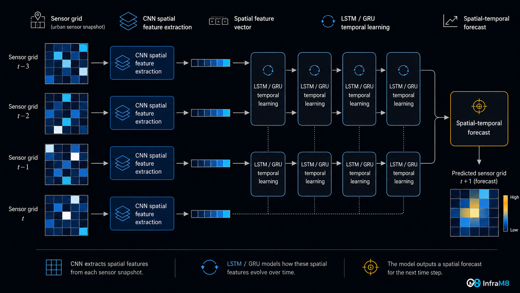
When sensor readings are assembled into a spatial matrix, with rows and columns representing geographic positions and cells containing measured values at a given time, the resulting structure is analogous to an image. CNN filters learn to detect local spatial patterns: a pollution gradient along a road corridor, a heat signature in a low-vegetation zone, a congestion cluster near an arterial junction. Hierarchical CNN layers extract progressively larger-scale spatial features [7].
Acknowledged limitations: Standard convolution assumes a regular Euclidean grid. Urban spatial relationships are frequently topological as well as Euclidean. Two points may be geographically close but effectively disconnected due to a barrier, a change in land use, or network topology. These limitations motivate graph-based approaches for problems where spatial relationships follow network topology [11], [12].
Long Short-Term Memory
Long Short-Term Memory networks, introduced by Hochreiter and Schmidhuber (1997), address a fundamental limitation of standard recurrent networks: the inability to retain relevant information across many time steps due to the vanishing gradient problem [2]. LSTMs achieve this through a gating mechanism with three components: an input gate controlling what new information enters the cell state, a forget gate controlling what is discarded, and an output gate controlling what is read to the hidden state [7].
In urban time-series contexts, LSTMs model temporal dependencies at multiple scales: capturing both the momentum of a current morning rush and the longer weekly cycle that distinguishes a Tuesday from a Saturday. Recent surveys of deep learning for temporal forecasting have documented LSTM-based architectures as among the most widely studied approaches across multiple forecasting domains [17].
Gated Recurrent Unit
Gated Recurrent Units, introduced by Cho et al. (2014), simplify the LSTM gating mechanism to two gates, a reset gate and an update gate, reducing the number of trainable parameters relative to LSTM [3].
Balanced comparison: The respective merits of LSTM and GRU are task- and data-dependent [7]. GRU's simpler gating structure may result in lower computational overhead in some deployment configurations, potentially making it more suitable for resource-constrained environments; however, this advantage is neither universal nor guaranteed, and empirical comparison on the specific task, dataset, hardware, and temporal horizon is always required. LSTM's additional expressiveness may be more useful when long-range temporal dependencies are important and sufficient training data is available. Neither architecture is universally superior; selection should be guided by comparative experiments rather than architectural assumption.
Table 1. Comparison of Architectural Components Used in Smart-City Spatial-Temporal Modeling
| Architecture | Main Role | Strengths | Limitations | Representative Smart-City Use Contexts |
|---|---|---|---|---|
| CNN | Spatial feature extraction | Local pattern detection; parameter sharing across spatial positions; efficient on grid-like data | Assumes regular spatial grid; limited for irregular or graph-structured sensor networks [11], [12] | Pollution field analysis; traffic flow grid aggregation; urban heat zone mapping |
| LSTM | Temporal sequence modeling | Long-range memory via gating; models multi-scale temporal dependencies [2] | Higher parameter count than GRU; risk of overfitting on small datasets; computationally demanding at inference | Air quality time series; energy demand forecasting; equipment health monitoring [15], [16] |
| GRU | Temporal sequence modeling | Simpler gating than LSTM; potentially more computationally efficient in some configurations [3] | May be less expressive than LSTM for certain long-horizon tasks; empirical validation required | Traffic speed sequences; real-time sensor monitoring; latency-sensitive IoT deployments |
| CNN-LSTM | Spatial-temporal prediction | Combines spatial feature maps with long-range temporal memory; demonstrated in spatially structured prediction tasks [4] | High parameter count; computationally demanding; requires regular spatial grid representation | Multi-step air quality forecasting; urban heat trajectory; energy district profiling |
| CNN-GRU | Spatial-temporal prediction | Spatial feature extraction with simpler recurrent modeling; potentially lower inference overhead in some contexts | May trade expressiveness for efficiency on complex long-horizon tasks; empirical validation required | Near-real-time traffic monitoring; short-horizon load forecasting; IoT-based predictive maintenance |
Note
Performance in all cases depends on dataset quality, spatial and temporal resolution, sensor density, preprocessing choices, validation strategy, and deployment context. Neither LSTM nor GRU is universally superior, and neither CNN-LSTM nor CNN-GRU is the appropriate choice for all smart-city prediction tasks. Comparison with simpler baselines and graph-based architectures is recommended for each specific application.
Section 05
CNN-LSTM and CNN-GRU for Spatial-Temporal Urban Learning
The combination of CNN spatial feature extraction with LSTM or GRU temporal sequence modeling produces architectures that are structurally matched to the nature of urban phenomena [4], [7]. Urban systems do not merely have a spatial configuration at a single moment. They have a history of spatial configurations, a trajectory through a space of possible states that unfolds over time, shaped by processes operating at multiple scales simultaneously.
The conceptual operation is as follows. At each time step, CNN layers process the spatial snapshot, a grid of sensor readings at that moment, and produce a compact spatial feature representation encoding where the relevant patterns are and what their local structure looks like. The sequence of these spatial feature vectors, one per time step, is passed to LSTM or GRU layers, which model how those spatial patterns evolved over time [4]. The recurrent output is used to generate a prediction for a specified future time step or horizon.
CNN-LSTM and CNN-GRU allow urban systems to learn not only what changed, but where it changed and how it evolved over time.
The ConvLSTM architecture established by Shi et al. (2015), which integrates convolutional operations within the recurrent structure itself, demonstrated that spatially correlated sequences could be modeled more faithfully than by treating spatial and temporal processing as separate stages [4].
Important architectural caveats and comparisons: CNN-LSTM and CNN-GRU are useful tools for spatial-temporal prediction when urban data can be reasonably represented as structured spatial grids. They are not universally superior to alternatives. Graph-based architectures, including DCRNN [11] and STGCN [12], have demonstrated that modeling spatial relationships through network adjacency can be advantageous for problems where urban topology matters. For any production deployment, CNN-LSTM and CNN-GRU should be compared empirically against persistence baselines, ARIMA/SARIMA, linear regression, Random Forest, XGBoost, standard LSTM, standard GRU, and, where applicable, graph-based and transformer-based architectures [17]. A complex model that does not meaningfully outperform a well-engineered simpler baseline does not justify its computational cost.
Table 2. Smart-City Applications, Sensor Data, and Spatial-Temporal Dimensions
| Application | Typical Sensors / Data Sources | Spatial Dimension | Temporal Dimension | Relevance of CNN-LSTM / CNN-GRU |
|---|---|---|---|---|
| Air Quality Prediction | Fixed monitoring stations; low-cost sensor nodes; weather stations; satellite aerosol optical depth products | Pollution gradients across districts; proximity to roads, industry, vegetation; wind corridor effects | Daily peaks and troughs; seasonal variation; event-driven spikes; lag effects from source to receptor | Spatial pollutant fields evolve with meteorology; CNN captures field structure; LSTM/GRU models hourly-to-daily evolution [13] |
| Urban Heat Monitoring | Temperature and humidity sensors; infrared sensors; weather stations; satellite land surface temperature imagery | Surface temperature varies with land use, vegetation density, building stock, surface albedo | Daily thermal cycle (afternoon peak, nocturnal cooling); seasonal amplitude; delayed radiative effects | Thermal zones exhibit spatial and temporal structure well-matched to hybrid architectures; application is conceptually motivated and actively researched; benchmark literature is developing [5] |
| Traffic Forecasting | Loop detectors; radar and microwave sensors; cameras; GPS floating car data | Congestion propagates along road corridors; spillback from downstream bottlenecks; topology-dependent propagation [11], [12] | Morning and evening peaks; day-type variation; incident-driven disruption and recovery | Spatial correlation follows road network; grid-based CNN approximates this; LSTM/GRU models daily-weekly temporal cycles |
| Energy Demand Forecasting | Smart meters; substation monitoring; building management systems; grid sensors | Demand varies by district land use; clustering of residential, commercial, and industrial loads | Time-of-day peaks; temperature-demand coupling; workday vs. weekend patterns; seasonal drift | District-level demand maps evolve with time-of-day and weather; hybrid model can forecast spatial load distribution [15] |
| Predictive Maintenance | Vibration sensors; current and voltage monitors; temperature probes; acoustic emission sensors | Multi-sensor co-activation patterns within equipment or across distributed asset fleet | Gradual fault signature development over extended periods; transient anomalies | Multi-sensor spatial co-activation evolves over time; hybrid model can identify degradation trajectory [16] |
Section 06
Practical Smart-City Applications
Air Quality Prediction
Air quality is among the most extensively studied smart-city prediction problems using spatially distributed data. Pollutant concentrations, including PM2.5, PM10, NO2, O3, CO2, and CO, vary continuously across a city in patterns driven simultaneously by emission sources, meteorological conditions, chemical transformation, and topographic constraints [5]. No single monitoring station can represent city-wide air quality; spatial interpolation requires a model of how concentrations vary in relation to sources, terrain, and atmospheric conditions.
Zheng et al. (2015) demonstrated the feasibility of fine-grained urban air quality forecasting by integrating spatially distributed monitoring data with weather and traffic inputs, establishing that multi-source spatial data could support prediction across city grids [13]. Operationally significant considerations include sensor calibration management, missing data handling, and the inclusion of meteorological co-variates as model inputs, since wind direction and speed are primary determinants of how pollution propagates spatially.
Urban Heat Island Monitoring
Urban heat islands arise from the interplay of reduced vegetation cover, thermally massive surface materials, concentrated anthropogenic heat release from transportation and buildings, and reduced evaporative cooling in impervious-surface-dominated urban environments [5]. These factors produce localized thermal environments that can diverge substantially from regional meteorological conditions, creating spatially heterogeneous temperature fields with pronounced daily and seasonal temporal dynamics.
The structural features of urban heat, spatial heterogeneity shaped by land use, temporal periodicity shaped by the solar cycle, and the modulating effects of weather and seasonal patterns, are well-matched to the representational properties of spatial-temporal deep learning architectures. Temperature and humidity sensor networks, complemented by land use classifications, vegetation indices, and remote sensing products, provide the multi-source spatial data these architectures require.
This application is conceptually well-motivated. Deep learning methods for urban heat analysis are an active area of research, and hybrid spatial-temporal approaches are increasingly being explored in urban climate and remote sensing contexts. Benchmark results for CNN-LSTM and CNN-GRU applied specifically to urban heat island prediction vary by study design, data availability, and spatial resolution; readers seeking current empirical comparisons are encouraged to consult the recent literature in urban climatology, remote sensing, and smart infrastructure. This is a domain where the modeling foundations are mature, the application is urgent, and the empirical validation literature is actively developing.
Traffic Forecasting
Traffic forecasting is one of the most intensively studied spatial-temporal prediction problems in urban deep learning, and the domain has produced some of the most architecturally consequential work in the field [11], [12]. Road network state, characterized by measurements of vehicle speed, volume, and occupancy at detector locations, exhibits simultaneous spatial and temporal structure that makes it a natural test case for spatial-temporal architectures.
Spatially, road segments are not independent: congestion propagates upstream from bottlenecks, incidents cause rerouting, and the hierarchical structure of the road network determines which flows affect which corridors. Li et al. (2018) demonstrated that modeling the road network as a directed graph and applying diffusion-based convolution over that graph, combined with a recurrent encoder-decoder, improved traffic forecasting by representing spatial dependencies more faithfully than grid-based approaches [11]. Yu et al. (2018) similarly applied spectral graph convolution with gated recurrent units to traffic prediction [12]. For operational systems, traffic forecasts must include uncertainty quantification [9] to be actionable for routing and signal control applications.
Energy Demand Forecasting
Urban energy demand forecasting benefits directly from the combination of spatial and temporal modeling. Kong et al. (2019) demonstrated short-term residential load forecasting using LSTM recurrent networks, showing that deep sequential models could represent the complex temporal dependencies in building-level consumption data [15]. Extending this to a spatial-temporal framework using CNN-LSTM or CNN-GRU allows district-level demand maps to be modeled as evolving fields, enabling forecasts that are conditioned on both historical spatial patterns and temporal dynamics.
Predictive Maintenance of Urban Infrastructure
Urban infrastructure generates continuous operational sensor streams: vibration signatures, thermal readings, current and voltage measurements, acoustic emissions, and flow rates. Zhao et al. (2019) reviewed deep learning applications to machine health monitoring, demonstrating that neural architectures could extract complex fault signatures from multi-sensor vibration and acoustic data [16]. Applying CNN-LSTM or CNN-GRU to predictive maintenance treats multi-sensor time series from a piece of equipment as a spatial-temporal object: multiple sensors form the spatial dimension, and the time series forms the temporal dimension.
Section 07
The Architecture Behind the Model
Smart-city intelligence is not primarily a modeling problem. It is an infrastructure architecture problem.
A CNN-LSTM or CNN-GRU model is one component in a system, a chain of dependencies extending from physical sensors in the urban environment to the operational decisions the model's outputs are intended to support. Every link in that chain conditions the usefulness of the model at its center [5], [6], [8].
The infrastructure chain
sensors -> signal quality -> telemetry -> data pipelines -> infrastructure -> model -> uncertainty -> decision
Table 3. The Infrastructure Chain: From Sensor to Decision
| Layer | Purpose | Common Failure Modes | Mitigation Strategy |
|---|---|---|---|
| Sensors | Capture physical urban phenomena as measurable signals | Drift; calibration degradation; noise; physical damage; power loss; connectivity failure [6] | Regular calibration verification; co-location with reference instruments; redundant power; physical protection; maintenance schedules |
| Signal Quality | Validate, filter, and correct raw sensor output before ingestion | Uncorrected drift treated as valid; outliers passed through; noise treated as signal; completeness not monitored | Automated outlier detection; drift correction models; completeness monitoring; domain-knowledge validation rules |
| Telemetry | Transmit validated sensor data from field to collection infrastructure | Connectivity interruption; packet loss; clock desynchronization; protocol incompatibilities; buffer overflow | Buffering with retry logic; time-synchronization protocols; redundant connectivity paths; protocol-level acknowledgment [8] |
| Data Pipelines | Transform ingested streams into structured, clean, feature-enriched datasets | Preprocessing inconsistencies; temporal misalignment across sensors; feature leakage; schema drift | Version-controlled pipeline code; automated data quality checks; schema validation; temporal alignment logic; integration testing |
| Infrastructure | Provide compute, storage, networking, and platform services | Infrastructure configuration drift; availability failures; security vulnerabilities; cost overruns | Infrastructure as Code; automated testing; cost governance; security baseline enforcement; redundancy design [8] |
| Model | Learn spatial-temporal patterns from data and generate predictions | Overfitting to training distribution; stale model after distribution shift; silent performance degradation | Temporal train/test splits; baseline comparison; regular retraining; performance monitoring; ablation studies |
| Uncertainty | Represent and communicate the model's prediction confidence [9] | Point estimates presented without bounds; overconfident intervals; uncalibrated uncertainty estimates | Prediction intervals; Monte Carlo dropout [9]; ensemble methods; conformal prediction; empirical calibration checks |
| Decision | Use model outputs to support operational decisions by domain experts | Blind trust in model output; decisions made without human judgment; no protocols for high-uncertainty outputs | Human-in-the-loop workflows; uncertainty-annotated dashboards; decision rules tied to prediction confidence |
A model can only be as useful as the system that produces, moves, validates, stores, interprets, and operationalizes its signals.
Section 08
Edge AI and Cloud Infrastructure Considerations
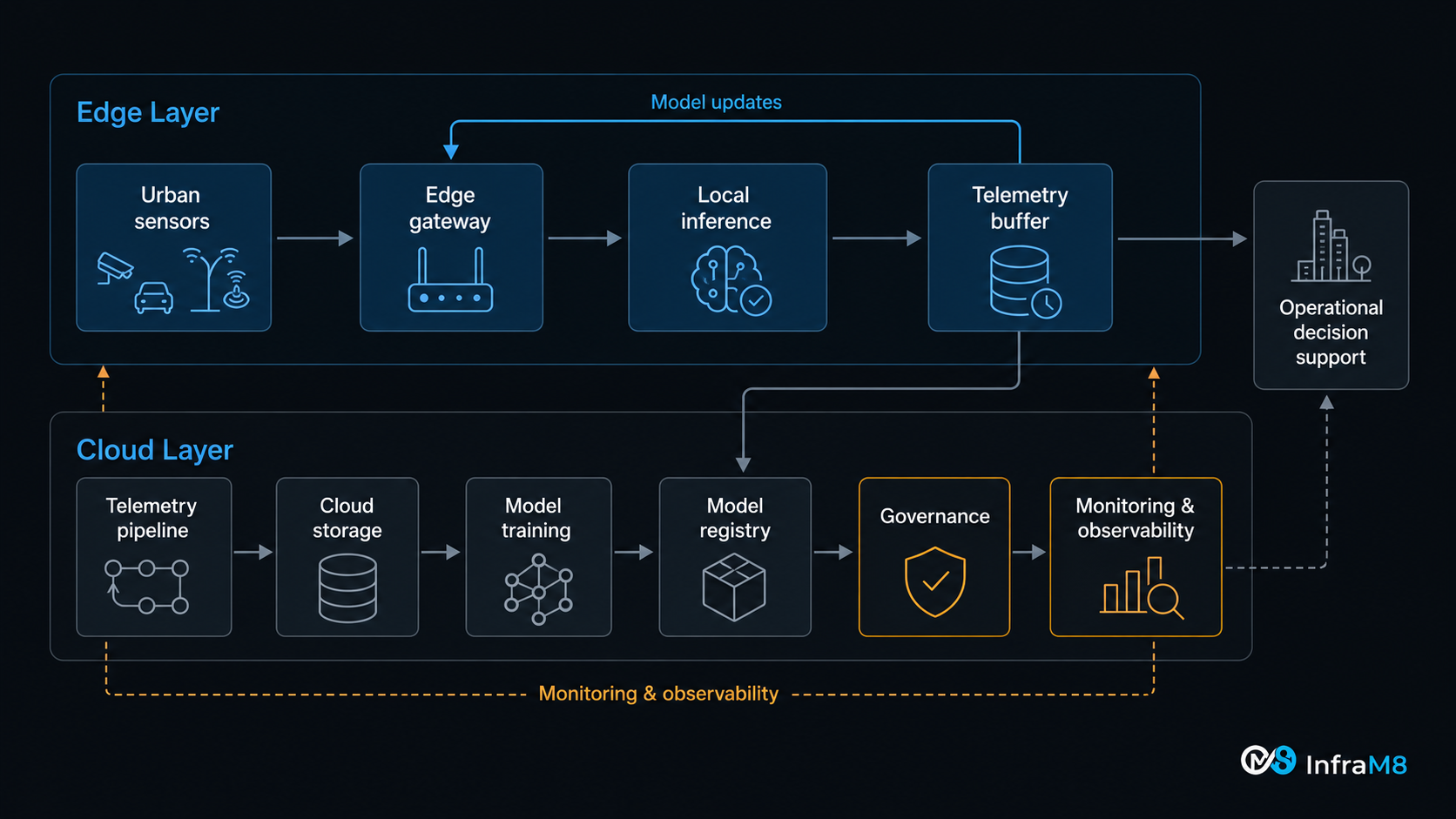
Deploying CNN-LSTM and CNN-GRU models in smart-city contexts involves infrastructure architecture decisions that extend beyond model design to the question of where computation happens: at the sensor edge, in a regional hub, or in centralized cloud infrastructure [8], [18].
Cloud infrastructure remains the standard environment for model training. The computational demands of training spatial-temporal models on multi-year, multi-site urban datasets are substantial, and cloud environments offer elastic compute, managed storage, data governance tooling, and the operational observability infrastructure needed for production workloads [8].
Edge inference becomes relevant when operational decisions require response times that cannot accommodate round-trip latency to cloud infrastructure, when network connectivity is intermittent or bandwidth-constrained, or when data sovereignty constraints limit raw sensor data transmission off-premises [8], [18]. Edge AI approaches involve deploying quantized, pruned, or otherwise compressed model variants on embedded processors or purpose-built inference accelerators located near sensors. The trade-off is reduced model expressiveness versus reduced latency and bandwidth requirements. Architectures with lower parameter counts, including CNN-GRU variants in some configurations, can be advantageous under specific edge constraints; however, this must be validated against the hardware profile, latency requirements, and accuracy thresholds of the specific deployment [18].
Hybrid cloud-edge architectures distribute responsibilities by latency and data sensitivity: edge nodes perform inference for time-critical decisions, buffer telemetry during connectivity windows, and report model performance metrics to cloud infrastructure; cloud infrastructure handles training, retraining triggered by detected drift, long-term storage, and governance functions [8].
Key operational considerations include model update cycles, observability, security baseline, and Infrastructure as Code. Edge-deployed models must be updated through tested, versioned, rollback-capable processes. Both edge inference performance and cloud pipeline health must be monitored continuously. Sensor endpoints and edge devices are attack surfaces, so authentication, data-in-transit encryption, and device attestation are security baselines. Infrastructure configuration should be defined in version-controlled, testable, declarative code because ad hoc changes are a primary source of irreproducibility and operational instability.
Section 09
Limitations and Risks
Responsible deployment of CNN-LSTM and CNN-GRU models in smart-city contexts requires honest assessment of their limitations and the operational risks they introduce [9], [14].
Data quality limitations. Models trained on sensor data affected by drift, missingness, or spatial coverage bias learn patterns that partially reflect measurement artifacts rather than urban phenomena. This failure mode is particularly insidious because the model continues producing outputs within superficially plausible ranges; the degradation is silent, not catastrophic [6].
Spatial coverage bias. If sensors are concentrated in high-income, high-visibility, or administratively convenient locations, the model's learned spatial representations will reflect those areas and may generalize poorly to undersampled districts [5]. Predictions for areas with sparse historical sensor coverage carry higher uncertainty that should be explicitly communicated.
Non-stationarity and concept drift. Urban systems change. Infrastructure is built and removed. Land use evolves. Mobility patterns shift in response to policy, technology, and events, as the COVID-19 period demonstrated starkly when pre-pandemic traffic and demand models produced unreliable outputs [14]. Models must be monitored for distributional shift, and retraining schedules should respond to detected drift rather than following fixed calendar intervals [14].
Overfitting. CNN-LSTM and CNN-GRU architectures have substantial capacity. On small or low-diversity training datasets, they can memorize training-set patterns that do not generalize to new periods or locations. Regularization, dropout, early stopping, and strict temporal holdout validation are essential practices.
Interpretability. Spatial-temporal deep learning models are largely opaque from the domain expert perspective. The features learned by CNN filters and the patterns encoded in recurrent states are not directly interpretable in terms of urban physics or engineering judgment.
A prediction without uncertainty can create false confidence. A point forecast produced without uncertainty representation implies a precision that the model almost certainly does not possess [9]. Operational systems that consume model outputs without uncertainty quantification may make allocation and intervention decisions based on false confidence, with potentially serious operational or public safety consequences. Monte Carlo dropout [9], ensemble methods, and conformal prediction provide practical frameworks for producing calibrated prediction intervals in deep learning forecasting systems.
Model transfer between cities. Urban spatial-temporal patterns are context-specific. A model trained on data from one city may not transfer reliably to another with different urban morphology, climate, mobility patterns, or sensor infrastructure. Transfer learning with local fine-tuning is preferable to direct application of models trained elsewhere.
Computational cost. Deep spatial-temporal models impose non-trivial computational costs at training and, in some configurations, at inference. This affects training frequency, retraining latency, inference throughput, and total operational cost, particularly in edge deployment contexts.
Table 5. Limitations, Risks, and Mitigation Strategies
| Risk | Why It Matters | Potential Impact on System | Mitigation Strategy |
|---|---|---|---|
| Sensor drift / poor calibration | Models train on biased signals and learn incorrect patterns [6] | Systematically biased predictions; decisions based on misrepresented ground truth | Regular co-location calibration; automated drift detection; quality flags propagated to training |
| Missing data | Gaps in sequences disrupt recurrent learning; biased pattern estimation | Degraded inference on incomplete inputs; silent errors during training | Imputation with uncertainty flagging; missingness features; completeness monitoring |
| Spatial coverage bias | Models reflect data-rich locations, not the whole city [5] | Predictions unreliable in undersampled districts; potential equity concerns | Document coverage gaps explicitly; amplify uncertainty for low-coverage zones; targeted sensor addition |
| Non-stationarity / concept drift | Urban dynamics change; static models become stale [14] | Accumulating forecast error after urban regime change; misleading predictions | Continuous performance monitoring; drift detection tests [14]; triggered retraining protocols |
| Overfitting | Complex models memorize rather than generalize | Good training metrics; poor field performance | Temporal holdout validation; regularization; dropout; preserved temporal ordering in cross-validation |
| No uncertainty quantification | Point forecasts imply false precision [9] | False operational confidence; missed risk signals | Monte Carlo dropout; ensemble methods; conformal prediction [9]; calibrated interval validation |
| Interpretability gap | Domain experts cannot audit what the model learned | Undetected physically implausible predictions; governance and accountability risk | Gradient-based attribution; attention visualization; domain expert review of edge case predictions |
| Inter-city transfer | Patterns in one city do not necessarily generalize to another | Deployed model underperforms; no local history to detect the gap | Domain adaptation; local fine-tuning on recent data; mandatory local validation before deployment |
| Infrastructure dependency | Model quality is bounded by all upstream pipeline stages | Best-case model performance limited by worst upstream failure mode [6] | End-to-end pipeline testing; infrastructure observability; data service-level agreements |
Section 10
Scientific and Practical Maturity Requirements
Deploying CNN-LSTM or CNN-GRU models in production smart-city systems requires scientific and engineering rigor that is not always present in proof-of-concept research demonstrations.
Baseline comparison is mandatory. Performance must be compared against: persistence forecasts, ARIMA/SARIMA, linear regression with temporal and spatial features, Random Forest, XGBoost, standard CNN, standard LSTM, and standard GRU. A complex spatial-temporal model that does not meaningfully outperform a well-engineered XGBoost baseline does not justify its computational and operational cost. In road network applications, comparison against graph-based models [11], [12] is also appropriate.
Temporal integrity of train/test splits. All training data must precede all test data chronologically. Cross-validation that randomly shuffles time steps violates temporal ordering and produces optimistic performance estimates that do not reflect true generalization to future periods. Rolling or expanding window validation is appropriate when multiple evaluation periods are required.
Spatial validation. Held-out spatial locations, sensors or zones not included in training, assess the model's ability to generalize spatially, not merely interpolate over trained locations.
Ablation studies. Testing CNN-only, LSTM/GRU-only, and full CNN-LSTM/CNN-GRU configurations reveals whether each architectural component contributes to performance, and whether the full complexity is justified by the data.
Uncertainty estimation. Production models must output prediction intervals, not only point estimates [9]. Prediction intervals must be empirically calibrated: a 90% prediction interval should contain the true value approximately 90% of the time on held-out test data.
Model and data drift monitoring. Deployed models must be monitored continuously for performance degradation [14]. Statistical process control, distributional shift tests, and automated alerts for accuracy degradation are operational requirements for any production deployment.
Reproducibility and documentation. Training procedures, preprocessing pipelines, hyperparameter configurations, and evaluation protocols must be documented and version-controlled. A model that cannot be reproduced cannot be audited, safely retrained, or defended in operational or regulatory contexts.
On alternative architectures. Graph Neural Networks and spatial-temporal graph architectures [11], [12] are better suited to problems where urban structure is inherently graph-based and topological fidelity matters. Transformer-based and attention architectures may offer advantages for long-horizon dependencies and multimodal forecasting tasks [17]. The choice of architecture should be governed by the structure of the problem, not by architectural reputation.
Table 4. Validation and Evaluation Checklist for Smart-City Spatial-Temporal Models
| Validation Area | Why It Matters | Recommended Practice | Example Metric or Method |
|---|---|---|---|
| Baseline comparison | Confirms complex model adds value over simpler approaches | Compare against persistence, ARIMA, XGBoost, standard LSTM/GRU | Error ratio: complex model vs. best simple baseline |
| Temporal train/test integrity | Prevents data leakage from future to past | Strict chronological split; no random shuffling of time steps | Confirm: no training data is later in time than any test data |
| Spatial holdout validation | Tests generalization to unseen locations | Hold out spatially distinct sensor zones from training | Error at held-out stations vs. error at trained stations |
| Rolling/expanding window CV | Realistic multi-period generalization estimate | Apply multiple non-overlapping train/test windows | Mean and variance of performance across evaluation windows |
| Ablation study | Understands contribution of each architectural component | Test CNN-only, LSTM/GRU-only, and full hybrid | Performance delta from removing each component |
| Uncertainty calibration | Ensures prediction intervals reflect true coverage probability [9] | Compute empirical coverage rate on held-out test set | 90% PI should cover truth about 90% of the time |
| Error analysis | Identifies systematic failure modes by condition | Segment residuals by time of day, day of week, season, weather | Residual plots by segment; high-error case review |
| Drift monitoring | Detects post-deployment performance degradation [14] | Track error on a rolling recent window vs. historical baseline | Rolling MAE; distributional shift tests; alert thresholds |
| Data quality audit | Ensures training data reflects physical reality | Review calibration logs; missing data rates; sensor quality history | Proportion of suspect readings; calibration deviation history |
| Reproducibility | Enables auditability and reliable retraining | Document all pipeline steps; version-controlled code and data | Can the model be independently retrained from documentation? |
Section 11
What This Means in Practice
Smart-city AI projects frequently begin with the model. They should begin with the infrastructure.
Before selecting an architecture, before training, before evaluating benchmark performance, a smart-city intelligence system requires honest answers to questions that determine whether any model can create operational value.
What is being sensed, and what does the sensor actually measure? The physical quantity of interest and the proxy signal produced by the sensor may diverge in ways that depend on ambient conditions, sensor aging, and installation context. Understanding this divergence is a prerequisite for evaluating data quality.
Where are the sensors placed, and what does that placement represent? Sensor placement driven by infrastructure access rather than statistical design creates spatial bias that propagates through the entire model. Knowing where sensors are not deployed is as important as knowing where they are.
How are signals calibrated, and how often? Calibration is a continuous operational function, not a one-time activity. A calibration strategy, including co-location schedules, reference instrument access, automated drift monitoring, and correction procedures, should be specified before a sensor network is considered production-ready [6].
How is missing data handled, and who decides? Missing data handling involves domain decisions, such as whether a gap during a storm is physically plausible and whether it should be imputed or flagged, as well as statistical ones. These decisions affect what the model learns and how it behaves at inference time.
What telemetry failure modes exist, and what happens during a failure? Telemetry failures are normal operating events. Systems must be designed with buffering, retry logic, failure detection, and completeness monitoring from the start [8].
How is uncertainty communicated in model outputs? A dashboard displaying a predicted value without a confidence interval is providing incomplete information. Uncertainty representation must be a first-class output requirement [9].
Who owns the operational decision, and what is their relationship to the model output? The model is a decision support tool, not a decision maker. Domain experts who act on model outputs must understand what those outputs mean, how confident they are, and when they should be overridden.
How will the model be monitored after deployment, and who is responsible? Deployed models degrade as urban systems change [14]. Monitoring requires designated ownership, defined alert thresholds, response protocols for detected drift, and a retraining cadence tied to the rate of change of the phenomena being modeled.
What happens when the model is wrong? Operational systems fail. The consequences of model failure, such as underestimated pollution, missed congestion, or overestimated maintenance interval, must be understood and planned for. Fallback logic, human override protocols, and post-failure review processes are operational design requirements, not afterthoughts.
Starting with these questions, rather than with architecture selection, is the single most important shift in how smart-city AI projects should be approached.
Section 12
Conclusion
A city does not behave like a spreadsheet. It behaves as a spatial-temporal system, continuously evolving across location, time, climate, infrastructure, mobility, and human activity. Smart-city intelligence that treats urban data as a collection of isolated numbers, stripped of spatial context and temporal trajectory, makes an assumption that urban physics does not support.
CNN-LSTM and CNN-GRU architectures are structurally relevant to urban prediction problems because they encode the two-dimensional character of urban phenomena directly in their design. Convolutional layers extract spatial features from distributed sensor readings across the city [1]. Recurrent layers model how those spatial patterns evolve over time [2], [3]. The combination produces models that represent not only the current state of an urban system, but its trajectory [4], [7].
Their practical relevance spans air quality forecasting [13], traffic prediction [11], [12], urban heat monitoring, energy demand forecasting [15], and predictive maintenance [16]. In each domain, the spatial-temporal structure of the phenomenon provides modeling signal that purely temporal or purely spatial approaches discard. They are, however, best understood as useful components of larger systems rather than solutions in themselves. Graph-based architectures [11], [12] and attention-based models [17] may be more appropriate choices in specific problem configurations, and empirical benchmarking against simpler baselines is always required.
The system is the whole chain: sensors -> signal quality -> telemetry -> data pipelines -> infrastructure -> model -> uncertainty -> decision.
Each link conditions every subsequent one [5], [6], [8]. Poorly calibrated sensors feed incorrect patterns into training data. Unreliable telemetry produces missingness that disrupts sequential learning. Models without uncertainty quantification produce outputs that cannot be appropriately weighted in operational decisions [9]. Infrastructure without observability conceals degradation until its consequences are already visible. Systems that do not equip domain experts to override model outputs responsibly are not decision support systems; they are liability generators.
Smart cities are intelligent infrastructure systems. Building them requires engineering discipline, infrastructure maturity, scientific rigor, and a realistic understanding of the distance between a model that performs well on a retrospective benchmark and a system that creates value under operational conditions, from the sensor in the street to the decision in the meeting room.
References
References
- [1] Y. LeCun, L. Bottou, Y. Bengio, and P. Haffner, "Gradient-based learning applied to document recognition," Proceedings of the IEEE, vol. 86, no. 11, pp. 2278-2324, Nov. 1998. DOI: 10.1109/5.726791
- [2] S. Hochreiter and J. Schmidhuber, "Long short-term memory," Neural Computation, vol. 9, no. 8, pp. 1735-1780, Nov. 1997. DOI: 10.1162/neco.1997.9.8.1735
- [3] K. Cho, B. van Merrienboer, C. Gulcehre, D. Bahdanau, F. Bougares, H. Schwenk, and Y. Bengio, "Learning phrase representations using RNN encoder-decoder for statistical machine translation," in Proc. Conf. Empirical Methods Natural Language Processing (EMNLP), Doha, Qatar, Oct. 2014. arXiv:1406.1078.
- [4] X. Shi, Z. Chen, H. Wang, D.-Y. Yeung, W. Wong, and W. Woo, "Convolutional LSTM network: A machine learning approach for precipitation nowcasting," in Advances in Neural Information Processing Systems (NeurIPS), vol. 28, Montreal, Canada, 2015. arXiv:1506.04214.
- [5] A. Zanella, N. Bui, A. Castellani, L. Vangelista, and M. Zorzi, "Internet of Things for Smart Cities," IEEE Internet of Things Journal, vol. 1, no. 1, pp. 22-32, Feb. 2014. DOI: 10.1109/JIOT.2014.2306328
- [6] A. Al-Fuqaha, M. Guizani, M. Mohammadi, M. Aledhari, and M. Ayyash, "Internet of Things: A survey on enabling technologies, protocols, and applications," IEEE Communications Surveys & Tutorials, vol. 17, no. 4, pp. 2347-2376, 2015. DOI: 10.1109/COMST.2015.2444095
- [7] I. Goodfellow, Y. Bengio, and A. Courville, Deep Learning. Cambridge, MA, USA: MIT Press, 2016. ISBN: 978-0-262-03561-3.
- [8] W. Shi, J. Cao, Q. Zhang, Y. Li, and L. Xu, "Edge computing: Vision and challenges," IEEE Internet of Things Journal, vol. 3, no. 5, pp. 637-646, Oct. 2016. DOI: 10.1109/JIOT.2016.2579198
- [9] Y. Gal and Z. Ghahramani, "Dropout as a Bayesian approximation: Representing model uncertainty in deep learning," in Proc. 33rd Int. Conf. Machine Learning (ICML), PMLR, vol. 48, pp. 1050-1059, New York, USA, 2016. URL: http://proceedings.mlr.press/v48/gal16.html
- [10] G. Atluri, A. Karpatne, and V. Kumar, "Spatio-temporal data mining: A survey of problems and methods," ACM Computing Surveys, vol. 51, no. 4, art. 83, Jul. 2018. DOI: 10.1145/3161602
- [11] Y. Li, R. Yu, C. Shahabi, and Y. Liu, "Diffusion convolutional recurrent neural network: Data-driven traffic forecasting," in Proc. 6th Int. Conf. Learning Representations (ICLR), Vancouver, Canada, 2018. arXiv:1707.01926.
- [12] B. Yu, H. Yin, and Z. Zhu, "Spatio-temporal graph convolutional networks: A deep learning framework for traffic forecasting," in Proc. 27th Int. Joint Conf. Artificial Intelligence (IJCAI), Stockholm, Sweden, pp. 3634-3640, 2018. arXiv:1709.04875.
- [13] Y. Zheng, X. Yi, M. Li, R. Li, Z. Shan, E. Chang, and T. Li, "Forecasting fine-grained air quality based on big data," in Proc. 21st ACM SIGKDD Int. Conf. Knowledge Discovery and Data Mining, Sydney, Australia, pp. 2267-2276, 2015. DOI: 10.1145/2783258.2788573
- [14] J. Lu, A. Liu, F. Dong, F. Gu, J. Gama, and G. Zhang, "Learning under concept drift: A review," IEEE Transactions on Knowledge and Data Engineering, vol. 31, no. 12, pp. 2346-2363, Dec. 2019. DOI: 10.1109/TKDE.2018.2876857
- [15] W. Kong, Z. Y. Dong, Y. Jia, D. J. Hill, Y. Xu, and Y. Zhang, "Short-term residential load forecasting based on LSTM recurrent neural network," IEEE Transactions on Smart Grid, vol. 10, no. 1, pp. 841-851, Jan. 2019. DOI: 10.1109/TSG.2017.2753802
- [16] R. Zhao, R. Yan, Z. Chen, K. Mao, P. Wang, and R. X. Gao, "Deep learning and its applications to machine health monitoring," Mechanical Systems and Signal Processing, vol. 115, pp. 213-237, Jan. 2019. DOI: 10.1016/j.ymssp.2018.05.050
- [17] B. Lim and S. Zohren, "Time-series forecasting with deep learning: A survey," Philosophical Transactions of the Royal Society A: Mathematical, Physical and Engineering Sciences, vol. 379, no. 2194, p. 20200209, 2021. DOI: 10.1098/rsta.2020.0209
- [18] S. Deng, H. Zhao, W. Fang, J. Yin, S. Dustdar, and A. Y. Zomaya, "Edge intelligence: The confluence of edge computing and artificial intelligence," IEEE Internet of Things Journal, vol. 7, no. 8, pp. 7457-7469, Aug. 2020. DOI: 10.1109/JIOT.2020.2984887